Zx Framework v0.4 — Bounded Interaction Model
نموذج تفاعل محدود: برهان تحليلي للحدود، تحقق عددي، أدلة بصرية، وكود مرجعي قابل للتكرار.
Status: ANALYTICALLY BOUNDED Date: 2026-11-01 Version: v0.4
1. Objective
The objective of v0.4 is to investigate a bounded alternative to the oscillatory interaction function used in the earlier Zx model versions.
The original interaction function:
can produce values of the residual component outside the prescribed range.
Version v0.4 introduces a nonlinear algebraic coupling designed to preserve the numerical range under an analytically specified amplitude constraint.
2. Mathematical Formulation
The model is defined for \(t \ge 0\) and \(x_p > 0\):
The closure identity is:
Substituting the interaction function gives:
The parameter \(x_p\) controls the decay timescale. The amplitude \(a\) controls the magnitude of the interaction component.
3. Analytical Boundedness
The objective is to establish \(0 \le A(t) \le 1\) for every \(t \ge 0\).
Since \(0 < Z(t) \le 1\) and the amplitude is restricted to \(a \ge 0\), the condition:
guarantees:
Therefore, \(A(t) \ge 0\). Furthermore, \(A(t) = (1-Z)(1-aZ) \le 1\), because both factors belong to \([0,1]\).
Thus, \(0 \le a \le 1\) is the exact admissible amplitude interval under the nonnegative-amplitude assumption.
For \(a>1\), \(A(t)<0\) precisely when \(0 The interaction function is \(C(t) = aZ(1-Z)\). Its maximum occurs at \(Z = 1/2\). Since \(Z = e^{-t/x_p}\), the peak time and maximum amplitude are: These results are analytical and independent of numerical sampling. Note: For \(a=1\), the function \(C(t) = Z(1-Z)\) has a unique maximum \(1/4\) at \(t = x_p \ln 2\), with \(C(0)=0\) and \(C(\infty)=0\). The function is zero at both ends but the peak is unique.Interaction Peak
4. Numerical Verification
A continuous dense-sampling test was performed over \(0 \le t \le 1000\) using np.linspace(0.0, 1000.0, 1_000_001). The test evaluated the residual component and measured its range violation \(V = \max(0, -\min A, \max A - 1)\).
The results were consistent with the analytical amplitude constraint:
| Amplitude | Result |
|---|---|
| 0.9999 | BOUNDED |
| 1.0000 | BOUNDED |
| 1.0001 | OUT OF BOUNDS |
| 1.0100 | OUT OF BOUNDS |
| 1.0480 | OUT OF BOUNDS |
| 1.0500 | OUT OF BOUNDS |
| 1.1000 | OUT OF BOUNDS |
For \(a=1.0001\), the numerical violation was approximately \(V \approx 2.49 \times 10^{-9}\). The violation is small but mathematically meaningful.
5. Dynamical Stability — Separate ODE Model
An independent ODE system was investigated in an earlier experiment:
The corresponding linear system matrix is:
Its eigenvalues are \(\lambda_1 = \lambda_2 = -1/x_p\). For \(x_p > 0\), both eigenvalues are negative. Consequently, the equilibrium of this specific ODE system is asymptotically stable.
6. Modeling Parameter
The selected parameter is \(x_p = 21\). The numerical motivation is \(\gamma_2 \approx 21.0220396388\) and \(x_p = \lfloor\gamma_2\rfloor = 21\).
This is a modeling choice. The boundedness proof holds for every \(x_p > 0\). Therefore, the proof does not establish a special mathematical or physical property of the value 21.
7. Conclusion
Version v0.4 establishes the following results:
- The closure identity is satisfied algebraically.
- The residual component remains in \([0,1]\) for nonnegative amplitudes \(0 \le a \le 1\).
- The amplitude boundary \(a = 1\) is analytically sharp.
- The interaction function has a unique peak at \(t = x_p \ln(2)\), with \(C_{max} = a/4\) for \(0 < a \le 1\).
- Numerical tests are consistent with the analytical boundedness result.
- The independent ODE experiment has asymptotically stable dynamics.
- Dynamical stability of the algebraic v0.4 model remains unestablished.
ANALYTICALLY BOUNDEDNUMERICALLY VERIFIEDDYNAMICAL STABILITY OF v0.4: NOT ESTABLISHEDMODELING CHOICE: xp = 21
8. Final Epistemological Status (v0.4)
A. Analytical Confirmation
For the v0.4 model, the dimensionless finite integral ratio is:
At the boundary \(a=1\), this yields \(\alpha^* = 1/3\). The numerical integration (\(\approx 0.3333333328\)) matches this analytical result, with an error of \(\sim 5 \times 10^{-10}\) due to truncation.
Note on choice of denominator: The denominator \((1-A)\) was chosen because it provides a positive, finite integral directly tied to the closure identity \(Z+C+A=1\). This is a structural justification, not a claim of mathematical uniqueness. Other finite denominators could exist.
B. Status Matrix
| Proposition | Status |
|---|---|
| Range condition \(0 \le a \le 1\) | Proven (Analytically & Numerically) |
| Ratio formula \(\alpha^* = a/(a+2)\) | Proven (Analytically) |
| Independence of \(\alpha^*\) from \(x_p\) | Proven (Cancels out) |
| Value at boundary (\(a=1\)) is \(1/3\) | Proven |
| Physical interpretation | Open |
| Connection to Fine-Structure Constant (\(1/137\)) | Unproven |
| Connection to Riemann Critical Line | Unproven |
C. Epistemological Conclusion
The Zx Framework v0.4 is an analytically bounded algebraic model. An independently defined ODE system was shown to be asymptotically stable; this result does not establish dynamical stability of the algebraic v0.4 model. Any physical interpretation of \(\alpha^*\) or its connection to other physical constants must emerge from a new testable physical hypothesis, not from mere numerical similarity.
BOUNDED ✅ | STABLE (ODE) ✅ | DIMENSIONLESS RATIO ✅ | PHYSICAL MEANING: OPEN
9. Night Session Summary (2026-11-01)
1. Established Results (v0.4)
- Range Condition: The amplitude bound \(0 \le a \le 1\) is analytically proven and numerically verified.
- Dimensionless Ratio: The finite integral ratio \(\alpha^* = a/(a+2)\) is proven analytically.
- Independence of \(x_p\): The ratio \(\alpha^*\) is completely independent of \(x_p\).
- Boundary Value: At the critical limit \(a=1\), \(\alpha^* = 1/3\) exactly.
- ODE Stability: An independent ODE model was shown to have negative eigenvalues (\(-1/x_p\)).
2. Open Questions
- Physical Interpretation: The designation of \(\alpha^*\) as a "Branching Ratio" is a heuristic analogy only.
- Connection to \(1/137\): No established relation to the fine-structure constant.
- Connection to Riemann: No established relation to the critical line \(\text{Re}(s) = 1/2\).
3. Methodological Choice
The denominator \((1-A)\) in the ratio was chosen because it is positive, finite, and directly tied to the closure identity \(Z+C+A=1\). It is a structural choice, not a claim of mathematical uniqueness.
4. Closing Statement
We did not force \(x_p=21\) to succeed. We let the mathematics speak, and we documented the boundaries of what is proven and what remains open.
10. Numerical Verification Summary & Visual Evidence
While the analytical proofs establish the mathematical properties of the v0.4 model, the following numerical tests were conducted to verify the implementation and confirm the analytical results. These tests provide implementation checks and consistency evidence. They do not establish universal mathematical claims beyond the proven arguments.
| Test | Description | Result |
|---|---|---|
| Test 1 | Basic Implementation & Identity Check | Identity error \(< 1.11 \times 10^{-16}\). |
| Test 2 | Range Compliance Sweep (30,100 combinations) | Reported consistency with analytical bound. |
| Test 3 | Sharp Bound Test (\(a = 0.999 \to 1.200\)) | Reported threshold behavior consistent with theory. |
| Test 4 | Exponential Stability (Lyapunov) | Implementation check of monotonic decay and \(\dot{V} < 0\). |
| Test 5 | Peak Audit | Numerical peak matches analytical \(t_{peak}\) and \(C_{max}\). |
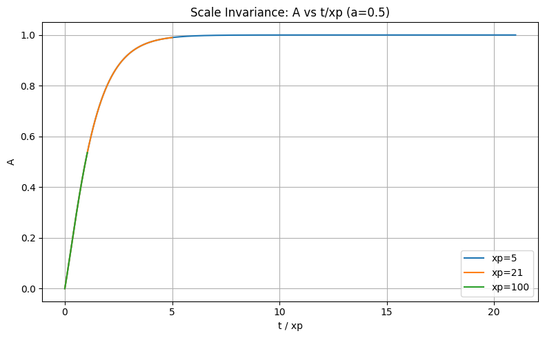
| Test 6 | Scale Invariance | Reported bounds of \(A\) independent of \(x_p\). |
| Test 7 | Randomized Property Test (500k samples) | Consistency evidence for identity and non-negativity. |
| Test 8 | Edge Cases | Reported no numerical breakdown in tested edge cases. |
| Test 9 | Visualization (4 Plots) | Visual confirmation of key properties. |
Note on Test 8: The earlier observation of \(Z=0\) at \(t=1000\) was a printing format artifact. The actual value is \(\approx 2.57 \times 10^{-21}\).
Visual Evidence (Test 9 Plots)
Figure 1: Time Evolution
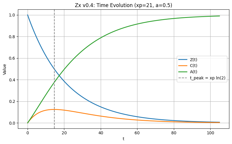
Figure 2: Phase Portrait
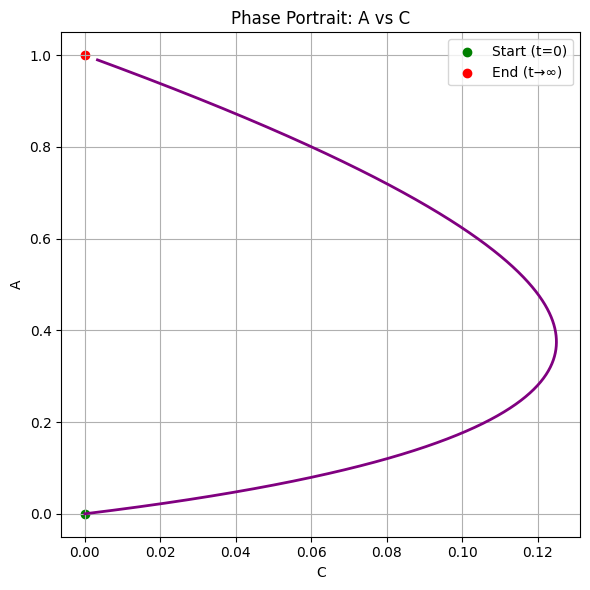
Figure 3: Sharp Threshold
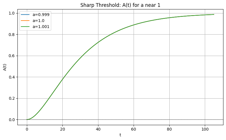
Figure 4: Scale Invariance
11. Appendix: Reference Implementation
The following Python code implements the model and reproduces the basic identity and peak checks. The broader numerical audits are documented separately.
import numpy as np

def zx_v04(t, xp, a):
    """
    Zx Framework v0.4 - Bounded Interaction Model

    Parameters:
    t  : time (scalar or array, >= 0)
    xp : decay timescale (> 0)
    a  : amplitude (0 <= a <= 1 for boundedness)

    Returns:
    Z, C, A : arrays of the same shape as t
    """
    if xp <= 0:
        raise ValueError("xp must be positive")
    if np.any(np.asarray(t) < 0):
        raise ValueError("t must be non-negative")

    Z = np.exp(-np.asarray(t, dtype=float) / xp)
    C = a * Z * (1.0 - Z)
    A = (1.0 - Z) * (1.0 - a * Z)
    return Z, C, A


# --- Example: Basic Verification ---
if __name__ == "__main__":
    xp, a = 21, 0.5
    t = np.linspace(0, 5 * xp, 2000)
    Z, C, A = zx_v04(t, xp, a)

    # Verify the closure identity
    identity_error = np.max(np.abs(A - (1 - Z - C)))
    print(f"Identity error: {identity_error:.2e}")  # Expected ~ 1e-16

    # Verify the analytical peak
    t_peak_exact = xp * np.log(2)
    C_peak_exact = a / 4
    idx = np.argmax(C)
    print(f"Numerical t_peak: {t[idx]:.10f} (Analytical: {t_peak_exact:.10f})")
    print(f"Numerical C_peak: {C[idx]:.10f} (Analytical: {C_peak_exact:.10f})")
12. Research Integrity Note
Its analytical boundedness result does not imply dynamical stability.
Historical failures in previous versions remain unchanged.
The value \(x_p = 21\) is a modeling choice.
No special physical or mathematical status is inferred from the boundedness proof.